1 Introduction to R & RStudio
Author: Alicia Johnson
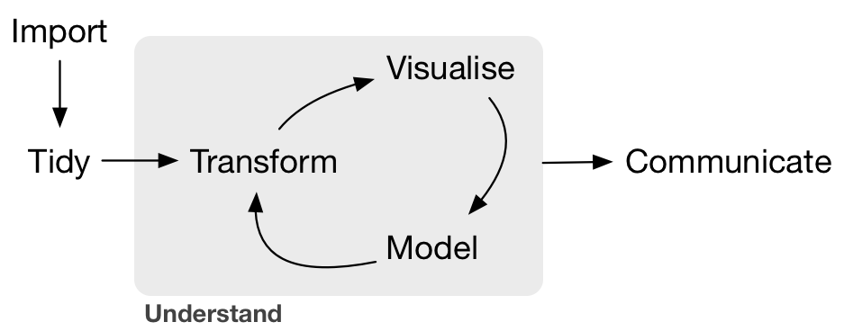
This workshop is motivated by the increasing need for tools that can be used to elucidate trends, decisions, and stories from data. This practice is broadly referred to as “data science”, a workflow for which is presented by Garrett Grolemund & Hadley Wickham:
Workshop Outline & Goals
Our goal is to provide a hands on introduction to navigating the data science pipeline with R and github. You will walk away with a solid foundation upon which you can build for your own research.
Day 1:
- Introduction to R & RStudio
- Data Visualization
- Simple Statistics
- Linear Regression
Day 2:
- Logistic regression
- Principles of Reproducible Research
- R Markdown
- Github in R
1.1 Getting Started
Whether your data are generated via simulation, collected via a survey, observed in a scientific experiment, scraped from the web, etc, you need software to explore and construct inferences from these data. In this workshop, we’ll use the R statistical software. Why R?
- it’s free
- it’s open source
- it’s flexible / useful for a wide variety of applications
- it has a huge online community
- it can be used to create reproducible documents, apps, books, etc. (In fact, this document was constructed within RStudio.)
Before the workshop, you were asked to download/update both R & RStudio:
Download & install R: https://mirror.las.iastate.edu/CRAN/
Download & install RStudio: https://www.rstudio.com/products/rstudio/download/
Be sure to download the free version. Note that RStudio is an integrated development environment (IDE) for R, combining the power of R with extra automation tools.
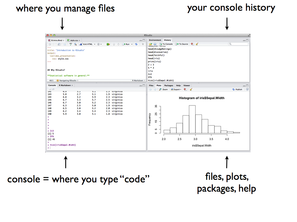
Once you open RStudio, you’ll see four panes, each serving a different function:
1.2 Basic features
Using R as a calculator
We can use R as a simple calculator. Try the following:
2 + 3
2 * 3
2^3
(2 + 3)^2
2 + 3^2
Comments
Once you start saving your work, it’s helpful to comment your code. To this end, R ignores anything after #.
# Calculate 3 squared
3^2
Built-in functions
R also includes built-in functions to which we supply arguments: function(arguments).
sqrt(9)

# The sum() function calculates the sum of the listed numbers
# Does the order of arguments matter?
sum(2, 3)
sum(3, 2)

# What does the rep() function do?
# Does the order of arguments matter?
rep(2, 3)
rep(3, 2)

# Arguments have names
rep(x = 3, times = 2)
rep(times = 2, x = 3)

# Is R case sensitive?  eg: Can we spell rep() as Rep()?
Rep(2, 3)
Assignment
We can assign & store R output.
# Store the result of rep(3, 2) as two_threes
two_threes <- rep(3, 2)

# Check out the results
two_threes

# Do something to the results
two_threes + 5

# Names cannot include spaces!
two threes <- rep(3,2)
1.3 Getting Help
Curious about what happens if you change R code in some way? Try it! Playing around with a function is the best way to learn about its functionality.
Can’t remember the code you used in a past analysis? Search for it under the “History” tab in the upper right hand panel in RStudio.
Did you make a mistake and don’t want to retype all of your work? Use the up arrow! You can access & subsequently edit any previous line of code by using the up arrow.
- Don’t know what a certain function does or how it works? You have a couple of options:
Use
?within RStudio to access help files.?rep- Google!
There’s a massive RStudio community at http://stackoverflow.com/. If you have a question, somebody’s probably already written about it.
1.4 Working with data
The following data were utilized in the fivethirtyeight.com article “The Dollar-And-Cents Case Against Hollywood’s Exclusion of Women” which analyzes movies that do/don’t pass the Bechdel test. Image from Wikipedia:
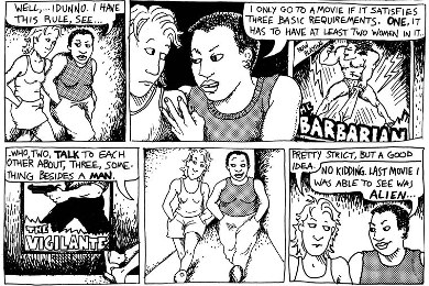
A movie passes the test if it meets the following criteria:
- there are \(\ge 2\) female characters
- the female characters talk to each other
- at least 1 time, they talk about something other than a male character
The fivethirtyeight analysis utilizes the following data:
Data Structure
Tidy data tables have two key features:
Each row represents a single observational unit of the sample.
Each column represents a variable, ie. an attribute of the cases.
The data are not treated like code. There are no extras - no row summaries, column summaries, data entry notes, comments, graphs, etc. All data manipulation should be done within R! All comments about the data collection, variables, etc should be provided in a separate code book.
Question: What are the units of observation in the above data? What are the variables?
Accessing / Importing Data
Data are stored in countless different locations (eg: your computer, Google drive, Wiki, etc) and in countless formats (eg: xls, csv, tables, etc). Luckily for us, the Bechdel data are already stored within R in the fivethirtyeight package. In general, packages developed & shared by R users provide specialized functions and data. IF AND ONLY IF you didn’t install the fivethirtyeight package before the workshop, you’ll need to do so now:
install.packages("fivethirtyeight", dependencies = TRUE)Once you install the package, you can load the package in your R session and access the bechdel data:
library(fivethirtyeight)
data(bechdel)
You can also access the codebook for these data:
?bechdel
Examining Data Structure in R
Before we do any data analysis we have to understand the structure of our data. Try the following.
# View the data table in a separate panel
View(bechdel)

# Check out the first rows in the console
head(bechdel)

# Obtain the data dimensions: rows x columns
dim(bechdel)

# Get the variable names
names(bechdel)
Examining Specific Variables
# Access a single variable using "$"
bechdel$budget_2013
bechdel$clean_test

# Determine levels/categories of categorical variables
levels(factor(bechdel$clean_test))
levels(factor(bechdel$binary))
Subsetting Specific Units of Observation
We can obtain a subset of observations that satisfy a criterion defined by a variable within the data set:
# Subset of movies with a 2013 budget under 1 million dollars
cheap <- subset(bechdel, budget_2013 < 1000000)
dim(cheap)
head(cheap)

# Subset of movies that fail the test
failures <- subset(bechdel, binary == "FAIL")
dim(failures)
head(failures)

# Subset of movies that EITHER have a budget under 1 million dollars OR fail the test
cheap_or_fail <- subset(bechdel, budget_2013 < 1000000 | binary == "FAIL")
dim(cheap_or_fail)
head(cheap_or_fail)

# Subset of movies that BOTH have a budget under 1 million dollars AND fail the test
cheap_and_fail <- subset(bechdel, budget_2013 < 1000000 & binary == "FAIL")
dim(cheap_and_fail)
head(cheap_and_fail)
Some useful syntax for subsetting:
<(less than),<=(less than or equal to),>(greater than),>=(greater than or equal to),==(equal to)&(and),|(or)
1.5 Exercises
Let’s apply the above tools to the US_births_2000_2014 data within the fivethirtyeight package. These data were used in the fivethirtyeight.com article “Some People Are Too Superstitious To Have A Baby On Friday The 13th”.
Load the data into your console and examine the codebook.
View the data set in a separate panel.
Check out the first 6 cases in your console.
What are the units of observation (rows)? What are the variables?
How much data do we have?
What are the names of the variables?
Access the
day_of_weekvariable alone. What are the levels/category labels for this variable?Create a subset that contains only the births that occur on Fridays. Store this as
OnlyFridays. Find the dimensions of this subset.Create a subset that contains only births in 2014. Store this as
Only2014. Find the dimensions of this subset.
Solutions:
#1
library(fivethirtyeight)
data(US_births_2000_2014)

#2
View(US_births_2000_2014)

#3
head(US_births_2000_2014)

#4
# Each row = a single day
# Variables include number of births, day of week, etc on that date

#5
dim(US_births_2000_2014)

#6
names(US_births_2000_2014)

#7
US_births_2000_2014$day_of_week
levels(factor(US_births_2000_2014$day_of_week))

#8
OnlyFridays <- subset(US_births_2000_2014, day_of_week == "Fri")
dim(OnlyFridays)

#9
Only2014 <- subset(US_births_2000_2014, year == 2014)
dim(Only2014)